comp_chem_utils

This directory contains the most important and fundamental modules of the comp_chem_py suite.

utils

Collection of simple functions useful in computational chemistry scripting.

Many of the following functions are used to make operations on xyz coordinates of molecular structure. When refering to xyz_data bellow, the following structures (also used in molecule_data) is assumed:

atom 1 label  and corresponding xyz coordinate
atom 2 label  and corresponding xyz coordinate
: : :
atom N label  and corresponding xyz coordinate

For example the xyz_data of a Hydrogen molecule along the z-axis should be passed as:

>>> xyz_data
[['H', 0.0, 0.0, 0.0], ['H', 0.0, 0.0, 1.0]]

vel_auto_corr(vel, max_corr_index, tstep)

Calculate velocity autocorrelation function.

Parameters:

• vel (list) – The velocities along the trajectory are given as a list of np.array() of dimensions N_atoms . 3.
• max_corr_index (int) – Maximum number of steps to consider for the auto correlation function. In other words, it corresponds to the number of points in the output function.

get_lmax_from_atomic_charge(charge)

Return the maximum angular momentum based on the input atomic charge.

This function is designed to return LMAX in a CPMD input file.

Parameters:charge (int) – Atomic charge. Returns:‘S’ for H or He; ‘P’ for second row elements; and ‘D’ for heavier elements.

get_file_as_list(filename, raw=False)

Read a file and return it as a list of lines (str).

By default comments (i.e. lines starting with #) and empty lines are ommited. This can be changed by setting raw=True

Parameters:

• filename (str) – Name of the file to read.
• raw (bool, optional) – To return the file as it is, i.e. with comments and blank lines. Default is raw=False.

Returns:

A list of lines (str).

make_new_dir(dirn)

Make new empty directory.

If the directory already exists it is erased and replaced.

Parameters:dirn (str) – Name for the new directory (can include path).

center_of_mass(xyz_data)

Calculate center of mass of a molecular structure based on xyz coordinates.

Parameters:xyz_data (list) – xyz atomic coordinates arranged as described above. Returns:3-dimensional np.array() containing the xyz coordinates of the center of mass of the molecular structure. The unit of the center of mass matches the xyz input units (usually Angstroms).

change_vector_norm(fix, mob, R)

Scale a 3-D vector defined by two points in space to have a new norm R.

The input vector is defined by a fix position in 3-D space fix, and a mobile position mob. The function returns a new mobile position such that the new vector has the norm R.

Parameters:

• fix (np.array) – xyz coordinates of the fix point.
• mob (np.array) – Original xyz coordinates of the mobile point.
• R (float) – Desired norm for the new vector.

Returns:

The new mobile position as an np.array() of dimenssion 3.

change_vector_norm_sym(pos1, pos2, R)

Symmetric version of change_vector_norm function.

In other word both positions are modified symmetrically.

get_rmsd(xyz_data1, xyz_data2)

Calculate RMSD between two sets of coordinates.

The Root-mean-square deviation of atomic positions is calculated as

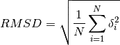
Where \delta_i is the distance between atom i in xyz_data1 and in xyz_data2.

Parameters:

• xyz_data1 (list) – List of atomic coordinates for the first structure arranged as described above for xyz_data.
• xyz_data2 (list) – Like xyz_data1 but for the second structure.

Returns:

The RMSD (float).

get_distance(xyz_data, atoms, box_size=None)

Calculate distance between two atoms in xyz_data.

Parameters:

• xyz_data (list) – xyz atomic coordinates arranged as described above.
• atoms (list) – list of two indices matching the two rows of the xyz_data for wich the distance should be calculated.

Returns:

Distance between the two atoms in the list as a float, the unit will match the input unit in the xyz_data.

get_distance_matrix(xyz_data, box_size=None)

get_distance_matrix_2(xyz_data1, xyz_data2, box_size=None)

get_angle(xyz_data, atoms)

Calculate angle between three atoms in xyz_data.

Parameters:

• xyz_data (list) – xyz atomic coordinates arranged as described above.
• atoms (list) – list of three indices matching the rows of the xyz_data for wich the angle should be calculated.

Returns:

Angle between the three atoms in the list as a float in degrees.

get_dihedral_angle(table, atoms)

Calculate dihedral angle defined by 4 atoms in xyz_data.

It relies on the praxeolitic formula (1 sqrt, 1 cross product).

Parameters:

• xyz_data (list) – xyz atomic coordinates arranged as described above.
• atoms (list) – list of 4 indices matching the rows of the xyz_data for wich the dihedral angle should be calculated.

Returns:

Dihedral angle defined by the 4 atoms in the list as a float in degrees.

conversions

Functions and constants to convert quantities from and to different units.

When executed directly, calls the two test functions:

• print_constants()
• test_conversion()

EV_TO_JOULES = 1.602176565e-19

Energy conversion from eV to J.

By definition an electron-volt is the amount of energy gained (or lost) by the charge of a single electron moving across an electric potential difference of one volt. So 1 eV is 1 volt (1 joule per coulomb, 1 J/C) multiplied by the elementary charge.

AU_TO_JOULES = 4.359744340736074e-18

Energy conversion from Hartree (a.u.) to J.

1 Hartree (a.u.) is defined as

CAL_TO_JOULES = 4.184

Energy conversion from cal to J.

1 calorie is defined as the amount of heat energy needed to raise the temperature of one gram of water by one degree Celsius at a pressure of one atmosphere. The thermochemical calorie (used here) is defined to be exactly 4.184 J.

KCALMOL_TO_JOULES = 6.947694845598683e-21

Energy conversion from kcal.mol-1 to J.

From the definition of the calorie.

AU_TO_KELVIN = 315775.04291721934

Conversions from a.u. to Kelvin when calculating kinetic temperature.

For a given kinetic energy in a.u. E_kin, we can obtain the kinetic temperature in Kelvin as:

Temp = 2.0 * E_kin * AU_TO_KELVIN / NDOF,

Where NDOF is the Number of Degrees Of Freedom.

AU_TO_S = 2.4188843280245007e-17

Time conversion from a.u. to seconds.

AU_TO_FS = 0.024188843280245006

Time conversion from a.u. to femto-seconds.

AU_TO_PS = 2.4188843280245007e-05

Time conversion from a.u. to pico-seconds.

BOHR_TO_ANG = 0.52917721092

Distance conversion from Bohr (a.u.) to Angstroms.

ATOMIC_MASS_AU = 1822.8884847700401

Atomic mass unit expressed in atomic units.

SPEC_TO_SIGMA = 1667562945278699.8

Conversion constant between a spectral function S expressed in seconds (reciprocal angular frequency unit) and the absorption cross section \sigma expressed in Angstroms^2.

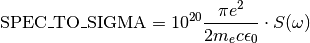
For more details see the documentation of the spectrum module.

SIGMA_TO_EPS = 26153.8273148873

Conversion constant between an absorption cross section \sigma expressed in Angstroms^2 and the extinction coefficient expressed in M^{-1} . cm^{-1}.

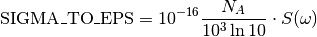
For more details see the documentation of the spectrum module.

convert(X, from_u, to_u)

Convert the energy value X from the unit from_u to the unit to_u.

Parameters:

• X (float) – Energy value to convert.
• from_u (str) – Unit of the input energy value X given as one of the keys of the dictionary convert_to_joules.
• to_u (str) – Unit of the output energy value X given as one of the keys of the dictionary convert_to_joules.

Returns:

The X value is returned expressed in the to_u unit.

Example

>>> from comp_chem_utils import conversions as c
>>> c.convert(1.0, 'WAVE LENGTH: nm', 'ENERGY: eV')
1239.8419292004205

test_conversion(value=1.0)

Use all possible conversions for a single value and printout the results.

This is intended as a test.

Parameters:value (float, optional) – hypothetical energy value. Default is 1.0.

print_constants()

Print all conversion constants defined in this module.

physcon

Library of physical constants.

This is coming from an old version of https://github.com/georglind/physcon.git

>>> import comp_chem_utils.physcon as pc
>>> pc.help()
Available functions:
[note: key must be a string, within quotes!]
  value(key) returns value (float)
  sd(key)    returns standard deviation (float)
  relsd(key) returns relative standard deviation (float)
  descr(key) prints description with units
:
Available global variables:
  alpha, a_0, c, e, eps_0, F, G, g_e, g_p, gamma_p, h, hbar, k_B
  m_d, m_e, m_n, m_p, mu_B, mu_e, mu_N, mu_p, mu_0, N_A, R, sigma, u
:
Available keys:
['alpha', 'alpha-1', 'amu', 'avogadro', 'bohrmagn', 'bohrradius', 'boltzmann', 'charge-e', 'conduct-qu', 'dirac', 'elec-const', 'faraday', 'gas', 'gfactor-e', 'gfactor-p', 'gravit', 'gyromagratio-p', 'josephson', 'lightvel', 'magflux-qu', 'magn-const', 'magnmom-e', 'magnmom-p', 'magres-p', 'mass-d', 'mass-d/u', 'mass-e', 'mass-e/u', 'mass-mu', 'mass-mu/u', 'mass-n', 'mass-n/u', 'mass-p', 'mass-p/u', 'nuclmagn', 'planck', 'ratio-me/mp', 'ratio-mp/me', 'rydberg', 'stefan-boltzm']

help()

Print information on how to use the module.

value(key)

Returns the value (float) of the physical constant corresponding to the input key.

Parameters:key (str) – single word description of an available constant. See help() to see available keys.

sd(key)

Returns the standard deviation (float) of the physical constant corresponding to the input key.

relsd(key)

Returns the relative standard deviation (float) of the physical constant corresponding to the input key.

descr(key)

Print a description of the physical constant corresponding to the input key.

spectrum

Collection of functions to read, calculate, and plot electronic spectra.

class Search(fname, search_str, col_id, offset=0, trim=(0, None), cfac=1.0)

Class for defining how to search spectrum information in an computational chemistry output file.

The information needed are excitation energies and oscillator strength. The assumption here is that in the output file this information can be located from a string search_str.

The data to be read can be shifted from the search_str by an offset number of lines. It is then found in a specific col_id inside the line which is splitted based on blank characters. It can be trimmed by trim and converted by cfac.

Example

Possible output file (named 'my_output'):

Excited State
E=1.0000cm-1 f=0.00000

In that case to extract the energy in eV we would have to do:

>>> from comp_chem_utils.spectrum import Search
>>> my_search_obj = Search('my_output', 'Excited State', 0, offset=1, trim=(2,7), cfac=1.2398e-4)
>>> my_search_obj.get_all()[0]
0.00012398

Parameters:

• fname (str) – Name of the output file containing the spectrum information. Can include path to file.
• search_str (str) – String that will be search in the output file to locate the data to be extracted.
• col_id (int) – The line matching the search string is splitted into a list with str.split() and the element col_id of the list is extracted.
• offset (int, optional) – In case the line of interest is not the line with search_str the offset can be used to shift to a line above (negative offset) or bellow the matching line. Default value is 0.
• trim (tuple) – In case the element col_id extracted from the line contains more than the desired data. A subset of the string can be extracted with trim. See example. Default is (0,None), i.e. it takes the whole element.
• cfac (float, optional) – In case the extracted data is not in the desired unit, it can be multiplied by cfac to convert it. Default value is 1.0.

get_all()

Extract all the relevant data depending on attribute values.

Returns:The extracted data is returned as floats in a 1-D np.array().

get_single(lines, idx)

Once a matching line has been located this method returns the associated data.

search_exc(kind, output)

Get excitation energies from an output file.

The kind of output file is used to determine the parameters to be used to set the Search class.

search_osc(kind, output)

Get oscillator strengts from an output file.

The kind of output file is used to determine the parameters to be used to set the Search class.

print_spectrum(exc_ener, strength, output)

Print table summary of Excitation energies and oscillator strengths.

read_spectrum(output, kind, verbose=False)

Read an output file and parse it to find excitation energies and oscillator strengths.

Note

If the spectrum data is written as a table, i.e. in the following format:

THIS IS A TABLE OF SPECTRUM DATA:
E (eV)     f
1.000    0.000
1.000    0.000
:        :

Then the read_table_spectrum() function should be used instead.

Parameters:

• output (str) – Name of the output file containing the spectrum information. Can include path to file.
• kind (str) – Kind of output, e.g. ‘gaussian’ or ‘lsdalton’. This is used in the search_exc() and search_osc() to set the parameters of the Search class. New kind have to be implemented in those functions.
• verbose (bool, optional) – If True the extracted data will be printed out. Default is False.

Returns:

exc, osc

Excitation energies and oscillator strengths are returned in the form of the two 1-D np.array(), exc and osc.

read_table_spectrum(output, search_str='', offset=0, pos_e=0, pos_f=1, verbose=False)

Read spectrum data arranged as a table in the output file.

Parameters:

• output (str) – Name of the output file containing the spectrum information. Can include path to file.
• search_str (str, optional) – String that will be search in the output file to locate the data to be extracted. If it’s not provided, the output is assumed to contain only raw data.
• offset (int, optional) – Number of lines to skip after the matching line before the table starts. Default is 0, which means that the table is assumed to start right after the matching line.
• pos_e (int, optional) – Column index for the excitation energies. Default is 0.
• pos_f (int, optional) – Column index for the oscillator strengths. Default is 1.
• verbose (bool, optional) – If True the extracted data will be printed out. Default is False.

Returns:

exc, osc

Excitation energies and oscillator strengths are returned in the form of the two 1-D np.array(), exc and osc.

spectral_function(exc, osc, unit_in='ENERGY: eV', nconf=1, fwhm=None, ctype='lorentzian', x_range=None, x_reso=None, raw=False)

Calculate the spectral function from theoretical data (excitation energies and oscillator strengths).

Note

It is not recommended to use this function directly. Instead the plot_spectrum() function should be used which serves as a wrapper and gives more flexibility on the output data.

The spectral function is calculated as

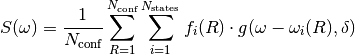
This expression is very well descrined in, e.g. [Barbatti2010a]. (f_i, omega_i) is the pair of input excitation energies and oscillator strengths, while omega is the incident frequency. The spectral line shape function is g which depends on the Full Width at Half Maximum delta, it is expressed in reciprocal angular frequency units, i.e. seconds (per molecules or structure).

Parameters:

• exc – Input excitation energies given in a one dimenssional np.array().
• osc – Input oscillator strengths given in a one dimenssional np.array().
• unit_in (str, optional) – String describing the unit used for the input excitation energies. The string must correspond to one of the keys of the dictionary convert_to_joules in the conversions module. Default is 'ENERGY: eV'.
• nconf (int, optional) – Total number of conformations used in the input data. This is used for normalization to a single structure. Default is 1.
• fwhm (float, optional) – Full width at Half Maximum used in the convolution function. It must be given in the same units as unit_in. The Default value is None, which will be latter changed to correspond to 0.1 eV.
• ctype (str, optional) – Defines the type of convolution. Either 'lorentzian' which is default or 'gaussian'.
• x_range (list, optional) – This is a two-value list defining the range of energy data for which the spectral function has to be calculated. It should be given in the same units as unit_in. It is default to None which will be latter changed to appropriate values related to the FWHM.
• x_reso (int, optional) – Resolution of the spectral function given as the number of grid points per energy unit (unit_in). The default value is None, which will be latter changed to correspond to 100 pts per eV.
• raw (bool, optional) – When True, the input excitation energies will not be converted to reciprocal angular frequency units. The output spectral function will thus be in reciprocal unit_in units and the user has to be careful for what is done to the output afterwards. The default is False.

Returns:

xpts, ypts

Those are two np.array() containing the grid points required to plot the spectral function. No matter the unit of the input energies, (unit_in). The spectral function (in ypts) is expressed in reciprocal angular frequency (seconds). While the xpts values are expressed in unit_in energy unit.

temperature_effect(E, unit_in='ENERGY: eV', temp=None)

Calculate tenperature factor for the absorption cross section.

The temperature effect is calculated as

where E is the input energy which will be converted to Joules.

Parameters:

• E (float) – Input energy or frequency expressed in unit_in.
• unit_in (str, optional) – String describing the unit used for the input excitation energies. The string must correspond to one of the keys of the dictionary convert_to_joules in the conversions module. Default is 'ENERGY: eV'.
• temp (float, optional) – Working temperature in Kelvin. The default value is None, which means that no temperature effect will be calculated.

Returns:

The temperature effect as a float. If temp=None, the value returned is 1.0.

cross_section(xpts, ypts, unit_in='ENERGY: eV', temp=None, refraction=1.0)

Calculate the absorption cross-section from the spectral function.

The cross section is just a scaled version of the spectral function that might depend on temperature and the refraction index of the medium.

Note

It is not recommended to use this function directly. Instead the plot_spectrum() function should be used which serves as a wrapper and gives more flexibility on the output data.

The xpts, and ypts input data are expected to come directly from a call to spectral_function().

Parameters:

• xpts (np.array) – Grid points corresponding to the x-axis of the spectral function. They are expressed in unit_in.
• ypts (np.array) – Grid points corresponding to the y-axis of the spectral function. They have to be given in reciprocal angular frequency units (seconds).
• unit_in (str, optional) – String describing the unit used for the input excitation energies. The string must correspond to one of the keys of the dictionary convert_to_joules in the conversions module. Default is 'ENERGY: eV'.
• temp (float, optional) – Working temperature in Kelvin. The default value is None, which means that no temperature effect will be calculated.
• refraction (float, optional) – The refraction index of the medium. Default value is 1.0.

Returns:

The absorption cross section is returned in Angstrom^2 . molecule^{-1}. It is calculated from the spectral function as

where the temp_effect comes from temperature_effect(), SPEC_TO_SIGMA is the main conversion constant from conversions, and n is the refraction index.

The absorption cross section is returned as grid points in an np.array().

plot_stick_spectrum(exc, osc, color=None, label=None)

Plot a stick spectrum from theoretical data.

The raw excitation energies and oscillator strength are used to make a stick spectrum.

The color and label arguments should be specified in order to ensure a uniform color for all the sticks.

Parameters:

• exc – Input excitation energies given in a one dimenssional np.array().
• osc – Input oscillator strengths given in a one dimenssional np.array().
• color (optional) – color code used in matplotlib.
• label (optional) – label to describe the data.

Returns:

Handle object comming out of the plt call that can be used for the legend.

plot_spectrum(exc, osc, unit_in='ENERGY: eV', nconf=1, fwhm=0.1, temp=0.0, refraction=1.0, ctype='lorentzian', x_range=None, x_reso=None, kind='CROSS_SECTION', with_sticks=False, plot=True)

Plot a spectrum based on theoretical data points.

This is the main function of the module that should be used to calculate and plot electronic spectra.

Parameters:

• exc – Input excitation energies given in a one dimenssional np.array().
• osc – Input oscillator strengths given in a one dimenssional np.array().
• unit_in (str, optional) – String describing the unit used for the input excitation energies. The string must correspond to one of the keys of the dictionary convert_to_joules in the conversions module. Default is 'ENERGY: eV'.
• nconf (int, optional) – Total number of conformations used in the input data. This is used for normalization to a single structure. Default is 1.
• fwhm (float, optional) – Full width at Half Maximum used in the convolution function. It must be given in the same units as unit_in. The Default value is None, which will be latter changed to correspond to 0.1 eV.
• temp (float, optional) – Working temperature in Kelvin. The default value is None, which means that no temperature effect will be calculated.
• refraction (float, optional) – The refraction index of the medium. Default value is 1.0.
• ctype (str, optional) – Defines the type of convolution. Either 'lorentzian' which is default or 'gaussian'.
• x_range (list, optional) – This is a two-value list defining the range of energy data for which the spectral function has to be calculated. It should be given in the same units as unit_in. It is default to None which will be latter changed to appropriate values related to the FWHM.
• x_reso (int, optional) – Resolution of the spectral function given as the number of grid points per energy unit (unit_in). The default value is None, which will be latter changed to correspond to 100 pts per eV.
• kind (str, optional) –

  String describing the type of spectrum that should be calculated. It has to be one of the following:

  'STICKS': 'Oscillator strength [Arbitrary units]',
  'SPECTRAL_FUNC': 'Spectral function [s. $\cdot $ molecules$^{-1}$]',
  'CROSS_SECTION': 'Cross section [$\AA^2 \cdot $ molecules$^{-1}$]',
  'EXPERIMENTAL': 'Molar absorptivity [M$^{-1}  \cdot $cm$^{-1}$]'
  

  The default is kind='CROSS_SECTION'.

• with_sticks (bool, optional) – If True, a stick spectrum will be plotted on top of what is required by the kind keyword. (Default is False). Will affect only when plot==True.
• plot (bool, optional) – To control wether to plot or not the spectrum. The default is to plot it.

Returns:

xpts, ypts

Those are two np.array() containing the grid points required to plot the desired spectrum. The xpts array contains the x-axis values in unit_in unit, while the ypts array contains the spectrum intensity with units depending on the chosen kind.

By default or if plot=True, the function will plot the desired spectrum and show it using the matplotlib tool.

cpmd_utils

Collection of functions to read and manipulate CPMD output files

read_standard_file(fn)

Read standard trajectory file and export it.

Here a trajectory file is understood as a file arranged as columns in which the first column contains the step indices and the others any type of informations.

For example the ENERGIES or SH_STATE.dat files enter in this category.

Parameters:fn (str) – Name of the trajectory file. Returns:steps, info

steps is as list of step indices (int) as read from the first column of the trajectory file, while info is an array (np.array()) of floats containing the rest of the information.

read_TRAJEC_xyz(fn)

Read TRAJEC.xyz file and export it.

An xyz type information is read for each step in the trajectory file, where xyz info is assumed to have the following format:

number of atoms
title line = step index
atom 1 label  and corresponding xyz coordinate
atom 2 label  and corresponding xyz coordinate
: : :
atom N label  and corresponding xyz coordinate

Parameters:fn (str) – Name of the TRAJEC.xyz file. Returns:steps, traj_xyz

steps (list): List of step indices (int) as read from

the title line of each xyz_data block.

traj_xyz (list): List of xyz_data blocks. Each block

is itself a list of the lines containing the coordinates in the xyz format. Each line is a 4 item list with first index the atom symbol and the last 3 items are the xyz coodinates.

read_GEOMETRY_xyz(fn)

Like read_TRAJEC_xyz for a single geometry and without the step index.

write_TRAJEC_xyz(steps, traj_xyz, output)

Write a TRAJEC.xyz file (CPMD style) to the output file.

Parameters:

• steps (list) – Step indices. See read_TRAJEC_xyz() function.
• traj_xyz (list) – xyz data. See read_TRAJEC_xyz() function.
• output (str) – Name (and path) fo the file in which the information will be written.

split_TRAJEC_data(steps, traj_xyz, verbose=True, interactif=True, write_xyz=False, start_i=1, nstep=100, delta=None, dt=5, name='')

Select equidistant xyz data snapshot from trajectory data.

From a starting index, a number of snapshots and a number of steps between each snapshot. A new trajectory data is generated with only a subset of steps.

Parameters:

• steps (list) – Step indices. See read_TRAJEC_xyz() function.
• traj_xyz (list) – xyz data. See read_TRAJEC_xyz() function.
• verbose (bool, optional) – Print more information while running. Default is True.
• interactif (bool, optional) – Let the user chose the parameters interactively. Default is True.
• write_xyz (bool, optional) – Write an xyz file to disk for every step. Default is False.
• start_i (int, optional) – Step index for the first snapshot. Default is 1
• nstep (int, optional) – Total number of final snapshots. Default is 100.
• delta (int, optional) – Number of steps between two snapshots. Default is None. It will be changed to the maximum possible value depending on other paramters.
• dt (int, optional) – Time step used in MD [in a.u.] (to provide print out the actual time between the snapshots). Default is 5 a.u.
• name (str, optional) – String/Title to be used in xyz filename in case write_xyz = True.

Returns:

new_steps, new_traj_xyz

Just a subset of steps and traj_xyz.

read_GEOMETRY(fn)

Simplified version of read_FTRAJECTORY for a single structure.

read_TRAJECTORY(fn, verbose=False)

Just a wrapper to read_FTRAJECTORY.

read_FTRAJECTORY(fn, forces=True, verbose=False)

Read the FTRAJECTORY file from a CPMD run and export it.

Three different formats can be read.

1. The TRAJECTORY file (with forces=False):

   Column 0: step index
   Column 1-3: xyz coordinates
   Column 4-6: velocities
   

2. The FTRAJECTORY file (with forces=True):

   Column 0: step index
   Column 1-3: xyz coordinates
   Column 4-6: velocities
   Column 7-9: forces
   

3. The FTRAJECTORYMTS file (with forces=True, this file is not produced anymore):

   Column 0: step index
   Column 1-3: low level forces
   Column 4-6: high level forces
   Column 7-9: xyz coordinates
   

read_ENERGIES(fn, code, factor=1, HIGH=True)

Read ENERGIES file from CPMD and return data based on code:

Parameters:

• fn (str) – filename of the ENERGIES file (can include path to the file).
• code –

  List of codes written as strings describing which information should be extracted from the file. The available codes are:

  'steps' : Step indices
  'E_kel' : Electronic kinetic energy (only for CPMD)
  'Temp'  : Temperature [K]
  'E_KS'  : Kohn-Sham energy [a.u.]
  'E_cla' : Classical energy, E_KS + E_kin (constant for BOMD)
  'E_ham' : 0 for BOMD
  'RMS'   : Nuclear displacement wrt initial position (?)
  'CPU_t' : CPU time
  

• factor (int) – Integer factor used to skip some information. E.g. for an MTS calculation the high level information can be extracted by setting factor equals to the MTS factor used in the calculation. Default value is 1 (every time step info is extracted).
• HIGH (bool) – define wether to extract the information every factor step (this is default, HIGH=True) or the negative counter part meaning the info is extracted for every step except every factor steps HIGH=False.

Returns:

The function returns a dictionary with keys the input codes and with values an array (np.array) containing the corresonding information as floats. The exception is the value for 'steps' which is a simple list of integers.

For example if the input codes are code=['steps','E_cla'], the output dictionary will have the form:

>>> read_ENERGIES('ENERGIES', ['steps','E_cla'])
{'E_cla': array([-546.99550862, -546.99770079, ..., -546.96549996]),
'steps': [1, 2, ..., 10000]}

read_SH_ENERG(fn, nstates=None, factor=1)

Read SH_ENERG.dat file and exctract info in dictionary

read_MTS_EXC_ENERG(fn, nstates, MTS_FACTOR, HIGH)

Read MTS_EXC_ENERG.dat file and exctract info in dictionary.

Either the HIGH or the LOW level info will be exctracted.

get_time_info(fn)

Read CPMD input file and extract time step info.

get_natoms(lines)

Get the number of atoms from a file like TRAJECTORY.

xyz_to_cpmd_atoms(xyz_data=None, xyz_filename=None, PPs=None)

Return list of strings as in CPMD ATOMS section.

qmmm_cpmd_atoms(atom_types, PPs=None)

Return list of strings as in CPMD ATOMS section for QMMM calculation.

xyz_data_to_np(xyz_data)

Convert xyz_data information to a tuple (atoms, coord)

Where atoms is a list of the atomic symbols and coord is a matrix: np.array[natoms, 3]

qmmm_utils

Set of routine to deal with xyz data of QMMM calculations.

In particular for solute/solvent system it is possible to extract a QM region based on a distance criterion from the solvent.

read_xyz_structure(xyz, nat_solute, nat_solvent)

decompose xyz data as solute + group of solvent molecules

get_distance(xyz_struc, ref)

For each block in xyz_struc, calculate distance to ref

get_QM_region(xyz, nat_slu, nat_sol, nmol_sol)

Extract QM information from the full set of coordinates.

The following structure is assumed:

First nat_slu atoms are the atoms of the solute molecules The rest are the solvent molecules arranged in blocks. For example, for a water solvent (nat_sol = 3):

O ...
H ...
H ...
O ...
H ...
H ...
:

Parameters:

• xyz (list) – xyz_data (list of list) for the whole system. Each sublist contains an atomic symbol and 3 (x,y,z) coordinates.
• nat_slu (int) – number of atoms of the solute molecule.
• nat_sol (int) – number of atoms of a single solvent molecule.
• nmol_sol (int) – total number of solvent molecules that should be included in the QM region.

Returns:

xyz_QM, atom_types, max_dist

xyz_QM (list): xyz_data for the QM region.

atom_types (dic): Each key is an atomic symbol and the

corresponding value is a list of indices of the atom of that type present in the QM region. The indices refer to the ordering of the original xyz_data.

max_dist (float): Distance (in AA) between the center of

mass of the solute and the center of mass of the farthest solvent molecule included in the QM region

mts_md_turbo

Multiple time step algorithm for Molecular Dynamics with Turbomole.

Default usage

The following files are required:

• GEOMETRY: a CPMD file for starting positions and velocities.

• define_high.inp: Input to TURBOMOLE’s define script to set up

  the high level electronic structure calculations.

• define_low.inp: same as define_high.inp but for low level.

From a python script or interpreter:

# setup the system, the list of atoms needs to be the same as in the GEOMETRY file.
system = system_settings(['O','H','H'])

# Run MD
data = md_driver(system)

The output dictionary data, contains the positions, velocities, forces, and energies along the MD trajectory.

The MD and TURBOMOLE parameters can be modified by setting the md_settings and turbo_settings objects and passing them to the md_driver.

class system_settings(atoms, linear=False)

class md_settings(max_iter=10000, time_step=10.0, mts_factor=1)

output()

class turbo_settings(high_input='define_high.inp', low_input='define_low.inp', nnodes=24)

load()

Load the environment necessary to run TURBOMOLE.

md_driver(sys_in, md_in=<comp_chem_utils.mts_md_turbo.md_settings object>, turbo_in=<comp_chem_utils.mts_md_turbo.turbo_settings object>)

Run a molecular dynamic using the RESPA algorithm of Tuckerman.

initialization(fname='GEOMETRY', nmts=1)

Initialize positions, velocities, forces, and energies.

The initial positions and velocities are read from a CPMD GEOMETRY file in atomic units. (Bohr not Angstrom!)

The Low and High level forces and energies are then calculated by calling the Turbomole program.

get_forces_and_energy(x, level)

Calculate forces and energies at a given level by calling TURBOMOLE.

vel_update(v, f)

Velocity Verlet update of Velocities.

data_update(data, x, v, f_low, f_high, e_low, e_high, idx, nmts)

Update the data dictionnary with the current iteration values.

The data are also written to disk.

write_xyz_data(fname, data, conv=1.0, nmts=1, idx=[])

Write or update XYZ type data to disk (positions, velocities, forces…).

write_energies(fname, E_pot, v, nmts=1, idx=[])

print to fname:

Step: MD step index (depends on nmts) E_pot: potential energy in a.u. E_kin: kinetic energy in a.u. E_tot: Constant energy (E_pot + E_kin) in a.u. Temp: Kinetic temperature in Kelvin

periodic

Simplified version of periodic table of atomic elements

class Element(mass, name, symbol, atomic)

Atomic elements are defined by mass, name, symbol, and atomic number.

type_(type_)

Returns a string representation of the ‘real type_’.

element(_input)

Takes periodic data as input, and returns the correct element.

molecule_data

Set of classes to deal with molecular data and formats

class mol_data

All information regarding a given molecule.

init_from_mol(mol_file)

update mol_data with data in mol (DALTON) format

init_from_xyz(xyz_file)

update mol_data with data in xyz format

init_from_db(cur, idd)

update mol_data with data from database

output()

return list of strings containing mol_data

out_to_mol()

generate mol_file data from mol_data

out_to_xyz()

generate xyz_file data from mol_data

out_to_db(cur)

add mol_data as a new entry to the molecules database

get_chem_name()

get/set chemical formula based on mol_data

check()

check consistency of mol_data

class atom_type

atom type as used in mol files (DALTON format)

to_angstrom()

convert coordinates from bohr to angstrom

read_from_mol(lines, iline, bohr)

return_xyz_table()

output(mol=False)

return list of strings as in mol file (Atomtypes section)

add_db_entry(cur, add_mol_xyz)

add xyz data as a new entry to the molecules database

set_from_GUI(atype_sec)

set atom_type information from GUI

class mol_file

structure and data of mol files (DALTON format)

check()

check consistency of mol_file

read_mol(filename)

update mol_file data from mol file

to_angstrom()

convert coordinates from bohr to angstrom

output()

return list of strings as in mol file

out_to_file(fname='')

class xyz_file

structure and data of xyz files

check()

check consistency of xyz_file

read_xyz(filename)

update xyz_file data from xyz file

read_from_table(table, fname='', title='')

xyz data is just a table with 4 columns and natoms lines

output()

return list of strings as in xyz file

out_to_file(fname='')

read_xyz_table(lines)

get_clean_atom_types(charges, xvals, yvals, zvals, bohr=False)

order and merge atom types

amino_acids

Just a dictionary of amino acids

pdbfile

Suppose to deal with pdb file format

class pdb_file

for now we assume a very simple structure: CRYST1 ATOM ATOM … END ATOM ATOM …

nstr()

change_atom(new_name, new_symb, old_name, old_symb)

change the atom name and symbol for a specific type of atom in the pdbfile

change_bond_length(atom_fix, atom_mob, R)

move atom_mob such that the distance to atom_fix is R

read(filen)

Read pdb file

output()

out_pdbfile(fn='')

keep_only(list_of_res)

delete all residues from the structures that dont belong to the list

class structure

for now we assume a structure is just a list of residues

nres()

change_atom(new_name, new_symb, old_name, old_symb)

change the atom name and symbol for a specific type of atom in the structure

change_bond_length(atom_fix, atom_mob, R)

move atom_mob such that the distance to atom_fix is R

read(lines, iline, name)

output()

keep_only(list_of_res)

delete all residues from the structure that dont belong to the list

get_list_of_res()

return list of residues in structure

export_xyz()

export xyz data as a 4 columns and natoms lines table

class residue

add_atom(atom)

change_atom(new_name, new_symb, old_name, old_symb)

change the atom name and symbol for a specific atom in the residue

rename_h_atoms()

change_bond_length(atom_fix, atom_mob, R)

move atom_mob such that the distance to atom_fix is R

read(lines, iline)

output()

class atom

read(line)

read line from pdb file that starts with ATOM and init atom type

update()

reconstruct self.line from data in atom

output()

return string to be printed as a line in a pdb file

class atom_name

read(name)

out()

get_res_num(line)

get residue number from line starting with ATOM

mysql_tables

Definitions of classes to work with molecular data.

The mol_info_table class is used to store and manipulated information about a molecule.

The mol_xyz_table class is used to store and manipulated the xyz coodinate of a molecule.

The functions defined here are basically wrappers to MySQL execution lines. Each function returns a MySQL command that should be executed by the calling routine.

mysql_add_row(table)

mysql_create_table(table)

class mol_info_table

handle the main database table mol_info

create_table()

find_duplicates(chem_name)

get_col(headers)

get_row(idd)

add_row()

delete_row(idd)

update(col, new, idd)

class mol_xyz_table(idd)

handle the coordinate database table mol_xyz

create_table()

get_table()

delete_table()

add_row()

program_info

class executable(prog, version=None)

This class is used to deal with available programs and their environments

get_exe()

get_env()

get_exec_line()

avail_progs()

choose_exec()

read_gaussian

This file contains a set of functions usefull to extract some information from Gaussian output files.

class gauss_atom

Contain basis information about an atom.

output()

get_gaussian_info(filename)

Extract relevant information from a Gaussian output file.

Goes through a gaussian output file looking for the information required to calculate PDOS.

Parameters:filename (str) – Name of the Gaussian output file, it may also include the path to the file. Returns:Number of occupied orbitals.

nbas (int): Number of basis functions (atomic orbitals).

overlap (np.array): Squared AO overlap matrix.

epsilon (list): Molecular orbital energies.

coef (np.array): Matrix of the molecular orbital coefficients.

Return type:nocc (int)

get_line(output, string)

Return the line number in ‘output’ containing the first occurence of ‘string’

read_triangular_matrix(start, dim, output)

read_triangular_block(iblock, dim, mat, iline, output)

read_orbitals_and_coefs(iblock, nbas, iline, ncol, epsilon, coef, output)

read_basis(iline, nbas, output)

read_atom_and_basis(gaussian_file)

read_boolean(string)

read boolean from users (yes/no question where yes is default)

sbatch_info

class sbatch_option

This class is used to deal with sbatch options

output()

detailed_output()

modify_from_user()

set_default(key)

set(value)

sbatch_line(script_name)

concatenate sbatch info into a submission line

References

[Barbatti2010a]

Barbatti, M. et al., (2010). The UV absorption of nucleobases: semi-classical ab initio spectra simulations. Physical Chemistry Chemical Physics, 12, 4959. http://doi.org/10.1039/b924956g